Food Justice NYC
Dionna Attinson, Arielle Coq, Martha Mulugeta, Tanu Sreedharan
Motivation
The motivation for this project stems from the fact that more than 1.2 million New York City (NYC) residents, or 14.4 percent, are experiencing food insecurity. Among residents in New York State, New York City residents make up half of all food insecure people. The rate of food insecurity in NYC is 12 percent higher than the national rate, and 21 percent higher than the New York State rate (Food Bank NYC, 2018).
Food insecurity has shown to have numerous effects on health outcomes and overall quality of life. Food insecurity is linked with poorer physical quality of life. An analysis on health indicators and food insecurity showed that communities with the highest rates of food insecurity face a higher prevalence for chronic diseases such as diabetes and obesity. This analysis also proved that those experiencing food insecurity have a higher incidence for other health-related metrics including lack of health insurance (Feeding America, 2018).
Related Work
In New York City, groups such as Hunger Free NYC, City Harvest, Food Bank for New York City, and the NYC Department of Health and Mental Hygiene are working towards providing more affordable, healthy food options to vulnerable groups.
Our work to synthesize data for this project highlighted the current gaps that exist in the data. For example, neighborhood-level data on the burden of food insecurity was difficult to access; much of the data identified was aggregated at the borough level. Further, many organizations studying food insecurity provide their findings in pdf reports, but not raw data for download.
Through this project, we hope to highlight the burden of food insecurity in NYC and the populations most affected, while also providing resources for those who can benefit from them.
Initial Questions
We sought to examine the relationship between food insecurity and physical/mental health-related outcomes. We also aimed to explore the prevalence of food insecurity in New York City and populations that are considered at-risk. Beyond simply describing food insecurity as a public health issue, we wanted to also provide a solution-oriented approach through the provision of resources that could help to address food insecurity. As such, our questions were as follows:
Data
For our food insecurity and chronic disease outcomes data, we utilized the The Community Health Survey.
For the resources dashboard, we used the following datasets to identify farmers markets, food banks, and community gardens across NYC:Exploratory Analysis
Loading and Tidying the Data
We were interested in food insecurity as a predictor to the following outcomes:The data for food insecurity and the chronic health outcomes of interest were obtained from the 2017 Community Health Survey. Obesity was defined such that participants with a BMI greater than or equal to 30 were considered obese. High blood pressure and diabetes status were determined from doctor, nurse, and/or health professional diagnoses. Lastly, the participants answered the 8-item Patient Health Questionnaire to diagnose current depression (last two weeks). We assessed the distribution of food insecurity and these chronic health outcomes by age, race, and sex.
As a means of tidying the original dataset, the variables were recoded so that a value of “1” indicated a case for each health outcome. These variables were also transformed from character to numeric to allow for further analysis, and they were renamed appropriately. The NAs were also dropped from the dataset to ensure we were looking solely at participants who had complete data.
Findings
The association between food insecurity and the select chronic health outcomes was assessed via logistic regression, adjusting for age categories, sex, and race categories.Age categories
Logistic Regression
Obesity \[ logit(Obesity) \sim \beta_0 + \beta_1 Food Insecure_i + \beta_2 Age_1i + \beta_3 Age_2i + \beta_4 Age_3i + \beta_5 Sex_i + \beta_6 Race_1i + \beta_7 Race_2i + \beta_8 Race_3i + \beta_9 Race_4i\]
data <- read_sas("data/chs2017_public.sas7bdat")

knitr::opts_chunk$set(
  echo = TRUE,
  warning = FALSE,
  fig.width = 8,
  fig.height = 6,
  out.width = "90%"
  )

options(
  ggplot2.continuous.colour = "viridis",
  ggplot2.continuous.fill = "viridis"
)

scale_colur_discrete = scale_colour_viridis_d
scale_fill_discrete = scale_fill_viridis_d

theme_set(theme_minimal() + theme(legend.position = "bottom"))

data_clean =
  data %>%
  select(imputed_foodinsecure, toldhighbp17, diabetes17, weight17in4, currdepress, agegroup, sex, newrace) %>%
  mutate(
    imputed_foodinsecure = recode(imputed_foodinsecure,
              "1" = "0",
              "2" = "0",
              "3" = "1",
              "4" = "1"),
    imputed_foodinsecure = as.numeric(imputed_foodinsecure),
    toldhighbp17 = recode(toldhighbp17,
                          "1" = "1",
                          "2" = "0"),
    toldhighbp17 = as.numeric(toldhighbp17),
    diabetes17 = recode(diabetes17,
                        "1" = "1",
                        "2" = "0"),
    diabetes17 = as.numeric(diabetes17),
    weight17in4 = recode(weight17in4,
                         "1" = "0",
                         "2" = "0",
                         "3" = "0",
                         "4" = "1"),
  weight17in4 = as.numeric(weight17in4),
    currdepress = recode(currdepress,
                         "1" = "1",
                         "2" = "0"),
  currdepress = as.numeric(currdepress),
    agegroup = recode(agegroup,
                      "1" = "18-24",
                      "2" = "25-44",
                      "3" = "45-64",
                      "4" = "65+"),
    sex = recode(sex,
                 "1" = "Male",
                 "2" = "Female"),
    newrace = recode(newrace,
                     "1" = "White non-Hispanic",
                     "2" = "Black non-Hispanic",
                     "3" = "Hispanic",
                     "4" = "Asian/PI/non-Hispanic",
                     "5" = "Other non-Hispanic"),
  ) %>%
  rename("Food_Insecure" = imputed_foodinsecure,
         "High_BP" = toldhighbp17,
         "Diabetes" = diabetes17,
         "Obesity" = weight17in4,
         "Depression" = currdepress,
         "Age" = agegroup,
         "Sex" = sex,
         "Race" = newrace) %>%
  drop_na()


fit_logistic_obesity =
  data_clean %>%
  glm(Obesity ~ Food_Insecure + Age + Sex + Race, data = ., family = binomial())

fit_logistic_obesity %>%
  broom::tidy() %>%
  mutate(OR = exp(estimate),
         High_CI = exp(estimate + 1.96*std.error),
         Low_CI = exp(estimate - 1.96*std.error)) %>%
  select(term, log_OR = estimate, OR, p.value, High_CI, Low_CI) %>%
knitr::kable(digits = 3)| term | log_OR | OR | p.value | High_CI | Low_CI |
|---|---|---|---|---|---|
| (Intercept) | -3.047 | 0.048 | 0.000 | 0.064 | 0.035 |
| Food_Insecure | 0.105 | 1.111 | 0.208 | 1.309 | 0.943 |
| Age25-44 | 0.692 | 1.998 | 0.000 | 2.514 | 1.587 |
| Age45-64 | 0.918 | 2.504 | 0.000 | 3.143 | 1.994 |
| Age65+ | 0.893 | 2.443 | 0.000 | 3.091 | 1.932 |
| SexMale | -0.142 | 0.868 | 0.004 | 0.956 | 0.787 |
| RaceBlack non-Hispanic | 1.703 | 5.490 | 0.000 | 6.896 | 4.371 |
| RaceHispanic | 1.647 | 5.194 | 0.000 | 6.503 | 4.148 |
| RaceOther non-Hispanic | 1.291 | 3.637 | 0.000 | 5.217 | 2.536 |
| RaceWhite non-Hispanic | 1.005 | 2.732 | 0.000 | 3.428 | 2.178 |
High Blood Pressure \[ logit(HighBloodPressure) \sim \beta_0 + \beta_1 Food Insecure_i + \beta_2 Age_1i + \beta_3 Age_2i + \beta_4 Age_3i + \beta_5 Sex_i + \beta_6 Race_1i + \beta_7 Race_2i + \beta_8 Race_3i + \beta_9 Race_4i\]
fit_logistic_High_BP =
  data_clean %>%
  glm(High_BP ~ Food_Insecure + Age + Sex + Race, data = ., family = binomial())

fit_logistic_High_BP %>%
  broom::tidy() %>%
  mutate(OR = exp(estimate),
         High_CI = exp(estimate + 1.96*std.error),
         Low_CI = exp(estimate - 1.96*std.error)) %>%
  select(term, log_OR = estimate, OR, p.value, High_CI, Low_CI) %>%
knitr::kable(digits = 3)| term | log_OR | OR | p.value | High_CI | Low_CI |
|---|---|---|---|---|---|
| (Intercept) | -3.506 | 0.030 | 0.000 | 0.043 | 0.021 |
| Food_Insecure | 0.441 | 1.555 | 0.000 | 1.842 | 1.312 |
| Age25-44 | 1.014 | 2.756 | 0.000 | 3.893 | 1.951 |
| Age45-64 | 2.442 | 11.498 | 0.000 | 16.104 | 8.209 |
| Age65+ | 3.616 | 37.193 | 0.000 | 52.406 | 26.396 |
| SexMale | 0.116 | 1.123 | 0.022 | 1.240 | 1.017 |
| RaceBlack non-Hispanic | 0.930 | 2.534 | 0.000 | 3.059 | 2.100 |
| RaceHispanic | 0.671 | 1.957 | 0.000 | 2.356 | 1.625 |
| RaceOther non-Hispanic | 0.685 | 1.984 | 0.000 | 2.802 | 1.404 |
| RaceWhite non-Hispanic | 0.100 | 1.106 | 0.279 | 1.326 | 0.922 |
Depression \[ logit(Depression) \sim \beta_0 + \beta_1 Food Insecure_i + \beta_2 Age_1i + \beta_3 Age_2i + \beta_4 Age_3i + \beta_5 Sex_i + \beta_6 Race_1i + \beta_7 Race_2i + \beta_8 Race_3i + \beta_9 Race_4i\]
fit_logistic_Depression =
  data_clean %>%
  glm(Depression ~ Food_Insecure + Age + Sex + Race, data = ., family = binomial())

fit_logistic_Depression %>%
  broom::tidy() %>%
  mutate(OR = exp(estimate),
         High_CI = exp(estimate + 1.96*std.error),
         Low_CI = exp(estimate - 1.96*std.error)) %>%
  select(term, log_OR = estimate, OR, p.value, High_CI, Low_CI) %>%
knitr::kable(digits = 3)| term | log_OR | OR | p.value | High_CI | Low_CI |
|---|---|---|---|---|---|
| (Intercept) | -2.637 | 0.072 | 0.000 | 0.102 | 0.050 |
| Food_Insecure | 1.487 | 4.422 | 0.000 | 5.291 | 3.695 |
| Age25-44 | -0.202 | 0.817 | 0.178 | 1.096 | 0.609 |
| Age45-64 | 0.033 | 1.034 | 0.820 | 1.378 | 0.776 |
| Age65+ | 0.195 | 1.215 | 0.201 | 1.637 | 0.902 |
| SexMale | -0.264 | 0.768 | 0.000 | 0.890 | 0.663 |
| RaceBlack non-Hispanic | 0.190 | 1.209 | 0.187 | 1.603 | 0.912 |
| RaceHispanic | 0.512 | 1.668 | 0.000 | 2.174 | 1.280 |
| RaceOther non-Hispanic | 0.728 | 2.071 | 0.001 | 3.241 | 1.324 |
| RaceWhite non-Hispanic | 0.202 | 1.224 | 0.144 | 1.607 | 0.933 |
Diabetes \[ logit(Diabetes) \sim \beta_0 + \beta_1 Food Insecure_i + \beta_2 Age_1i + \beta_3 Age_2i + \beta_4 Age_3i + \beta_5 Sex_i + \beta_6 Race_1i + \beta_7 Race_2i + \beta_8 Race_3i + \beta_9 Race_4i\]
fit_logistic_Diabetes =
  data_clean %>%
  glm(Diabetes ~ Food_Insecure + Age + Sex + Race, data = ., family = binomial())

fit_logistic_Diabetes %>%
  broom::tidy() %>%
  mutate(OR = exp(estimate),
         High_CI = exp(estimate + 1.96*std.error),
         Low_CI = exp(estimate - 1.96*std.error)) %>%
  select(term, log_OR = estimate, OR, p.value, High_CI, Low_CI) %>%
knitr::kable(digits = 3)| term | log_OR | OR | p.value | High_CI | Low_CI |
|---|---|---|---|---|---|
| (Intercept) | -4.640 | 0.010 | 0.000 | 0.019 | 0.005 |
| Food_Insecure | 0.399 | 1.491 | 0.000 | 1.823 | 1.220 |
| Age25-44 | 1.291 | 3.638 | 0.000 | 7.189 | 1.841 |
| Age45-64 | 2.824 | 16.851 | 0.000 | 32.759 | 8.668 |
| Age65+ | 3.642 | 38.151 | 0.000 | 74.269 | 19.598 |
| SexMale | 0.233 | 1.262 | 0.000 | 1.432 | 1.113 |
| RaceBlack non-Hispanic | 0.371 | 1.449 | 0.002 | 1.822 | 1.152 |
| RaceHispanic | 0.332 | 1.394 | 0.004 | 1.749 | 1.111 |
| RaceOther non-Hispanic | 0.315 | 1.370 | 0.153 | 2.110 | 0.890 |
| RaceWhite non-Hispanic | -0.627 | 0.534 | 0.000 | 0.674 | 0.423 |
Below are the summary measures of association corresponding to each regression model.
oddsratios_full = tibble(
  outcome = c("Obesity", "High BP", "Depression", "Diabetes"),
  OR = c(1.111, 1.555, 4.422, 1.491),
  pvalue = c(0.208, 0.000, 0.000, 0.000),
  Low_CI = c(0.943, 1.312, 3.695, 1.220),
  High_CI = c(1.309, 1.842, 5.291, 1.823))

oddsratios_full %>%
  ggplot(aes(x = OR, y = outcome, group = 1)) +
  geom_vline(aes(xintercept = 1), linetype = "dashed") +
  geom_errorbarh(aes(xmax = High_CI, xmin = Low_CI), size = 0.5, height = 0.2) +
  geom_point(size = 3.5, color = "orange") +
  ylab("") +
  xlab("Odds Ratio") +
  ggtitle("Food insecurity and odds of select outcomes") +
  labs(
    caption = "Data from Community Health Survey (2017)"
  )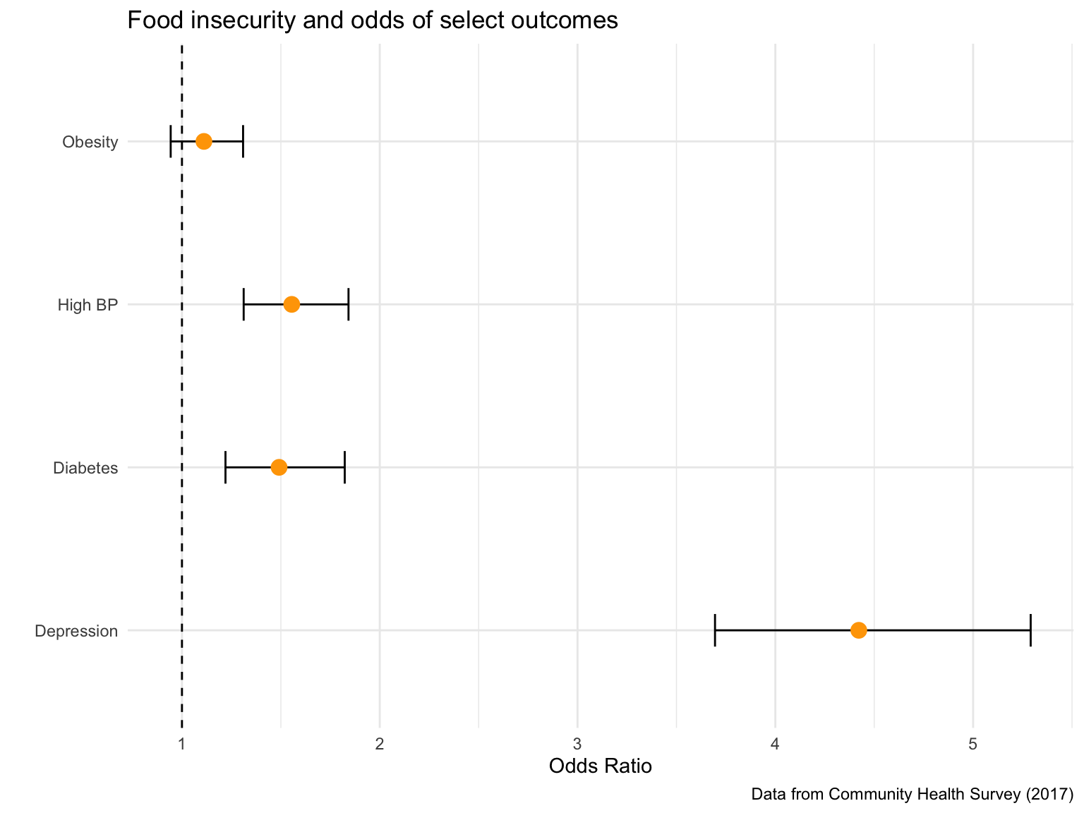
We found that the association was statistically significant for high blood pressure (OR = 1.555, 95% CI: 1.312-1.842), diabetes (OR = 1.491, 95% CI: 1.220-1.823), and depression (OR = 4.422, 95% CI: 3.695-5.291). However, the association was not significant for obesity (OR = 1.111, 95% CI: 0.943-1.309).
Additional Analysis
Geocoding
Food Insecurity Rate
We used the leaflet package to perform visualization of the geographic distribution of food insecurity in New York City. We observed that the highest rates food insecurity were observed in the Bronx (16%) and Brooklyn (17.1%). The lowest rate of food insecurity was observed in Staten Island (8.6%). This data is visually represented in the map and the table below.
| Borough | Food Insecurity Rate |
|---|---|
| Bronx | 0.16% |
| Brooklyn | 0.171% |
| Manhattan | 0.126% |
| Queens | 0.105% |
| Staten Island | 0.086% |
Spatial Visualization of Food Insecurity Rate by Borough in NYC
Food Resources
We used the leaflet package to perform visualization of geographic distribution of resources to address food insecurity in New York City.